Background Removal Using the Autobk Algorithm

The Autobk algorithm is the background removal method used in Ifeffit and, by extension, in Athena. The fundamental principle of this algorithm is that the background function μ₀(E) can be distinguished from the fine structure function χ(k) using a criterion defined in the space of the Fourier transform of χ(k). In short, we assert that there is a cut-off in R-space below which the Fourier components are dominated by the background and above which the Fourier components are dominated by χ(k).

The reference for the Autobk algorithm is here: DOI:10.1103/PhysRevB.47.14126

The default values for the background removal parameters

Here are some Ga K-edge data provided in a long-ago question on the Ifeffit mailing list. The background function, the red line, was determined using the default values for all the settings that effect its determination.

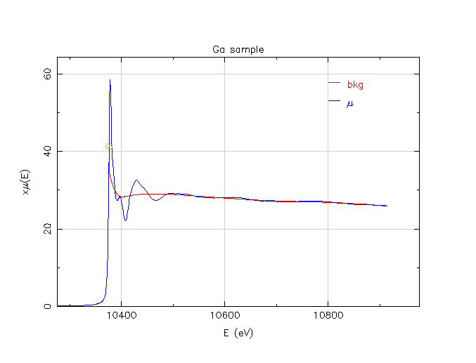
Ga μ(E) data with default background parameters

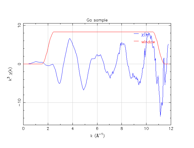
Ga χ(k) data with default background parameters

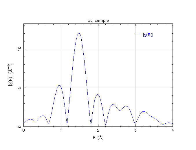
Ga χ(R) data with default background parameters

As you can see, the default values are not unreasonable. The μ₀(E) function doesn’t do anything too wacky, χ(k) looks like sine waves, and χ(R) has peaks in mostly reasonable locations.

That said, this data processing effort is not perfect, either. The χ(k) data about about 11 Å^-1 is kind of funny looking. Also, there is a peak just below 1 Å in χ(R) that is probably spurious. (Well, the fellow asking the question on the mailing list implied that he does not expect to see a peak at such a low R value. So I am presuming that the peak at about 1.5 Å represents the nearest neighbor.)

To proceed from here, one must understand which parameters in Athena affect the background removal and how they do so.

The background removal parameters

Here is a screenshot of Athena with several of its parameters highlighted. All the parameters in the “Background removal” section have some impact on how the data are processed, but the ones highlighted have the most significant impact. Additionally, I have highlighted two of the parameters in the forward Fourier transform section. How these relate to the topic at hand will be discussed later.

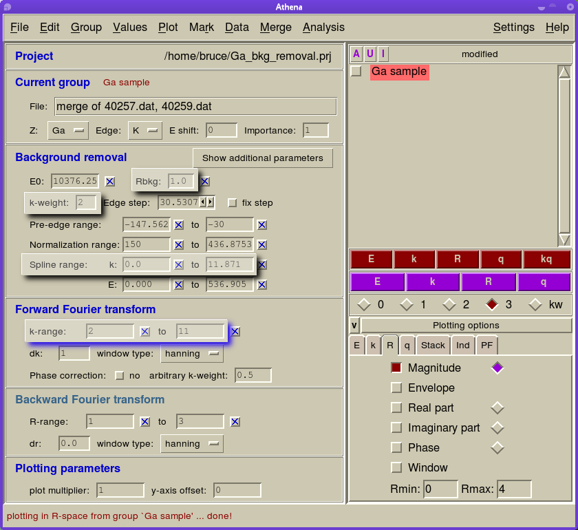
The Athena window with the most relevant parameters highlighted

To start, I’ll summarize the effect of the most important background removal parameters:

Parameter	Effect
Rbkg	This is the cutoff in R-space below which the Fourier components are understood to belong to the background function
k-weight	This is the k-weighting used in the Foruier transferm performed as part of the background refinement
spline range	This is the range in k-space over which the background function is evaluated

R_bkg

The function used to represent μ₀(E) is a simple spline. This spline has a number of variable parameters equal to the bandwidth of the signal used in its determination. What do I mean by bandwidth? It is a product of the range in k-space over which it is evaluated and the range in R-space to which it contributes spectral weight. Thus the spline has a limited number of parameters used in its evaluation and therefore a limit to how “wiggly” it can be. By limiting it’s range in R-space, it is prevented from having Fourier components that we consider to be due to χ(k). This the μ₀(E) function is “stiffer” or “smoother” than the μ(E) data such that, when it is subtracted from the measured data, the χ function is isolated.

By default, the value of R_bkg is 1 Å. That is, the default is to say that the Fourier components below R=1 Å are due to the background function. The Autobk algorithm works by refining the spline function such that, when subtracted from the data and Fourier transformed, the Foruier components below R_bkg are minimized.

A good rule of thumb is to make R_bkg about equal to half the near neighbor distance. If the neighbor is close (as for an oxide), R_bkg can be smaller. If the neighbor is farther away (as for a metal), R_bkg can be larger. If you make R_bkg too small, the spline will not have sufficient freedom to follow the shape of the μ₀(E) function. If you make R_bkg too large, you will be giving the spline sufficient freedom to follow the χ(k) function, thus subtracting it will damage the extracted χ(k).

k-weight

Implicit in the explanation of the R_bkg parameter is that a Fourier transform is done to determine the background function. More precisely, a Fourier transform is made as part of the optmization of the spline. Each time the spline parameters are changed during this optimization, a Foruier transform of the data is made. The k-weight in the background removal section is the value of k-weighting that is used in the Fourier transform performed repeatedly as part of the optimization of the spline. This is not the k-weighting that is used to visualize your data. When visualizing your data, the k-weight value selected from the strip just below the purple plot buttons is used. You are, therefore, able to process your data using one value of k-weight and visualize it with a different value. Or the same – your choice.

Why does it matter how the k-weight is set during the spline optimization? Well, the value of k-weight will have an impact on the size of the Fourier components below R_bkg. With a larger value of k-weight, the high-k portion of χ(k) will be enhanced. It will then, in a sense, enhance the sensitivity of the optimization to the the exact value of the spline at high k values.

In my experience, a k-weight of 3 for the background removal is a good choice for beautiful data, i.e. data that are not overly dominated by statistical or systematic error at high k value. For noisy data, a large valule of this k-weight can make the optimization unstable by forcing the spline to attempt to follow amplified noise. For noisier data, I find that a k-weight of 2 or even 1 is necessary.

spline range

Several mentions were made in the preceeding about the range of the spline (or equivalently, the range over which the Fourier transform is evaluated). That is set by these two parameters. The default in Athena is to evaluate the spline from 0 (i.e. from the edge energy) until the end of the data. If the end of the data is dominated by some systematic effect that dominates χ(k) (a really good example would be the presence of another absorption edge), then the spline can be truncated by setting the upper limit. In some case, the spline has trouble following the data near the edge, where the data are changing very rapidly. This might be a problem in the presence of a very pronounced white line. In that case, you can start the evaluation of the spline at a slightly higher energy, thus avoiding the most rapidly varying portion of the μ(E) data.

There is one more parameter that merits explanation. If you click the “Show additional parameters” button, you will see controls for the spline clamp. The spline clamps are a simple tool to constrain the ends of the spline to remain close to the μ(E) data. At times, the optimization of the spline might be such that the ends deviate significantly from the data. This would be a numerical result. Physically speaking, μ₀(E) should always more or less “bisect” the wiggles of μ(E). The clamps work by adding a penalty to the metric that is evaluated in the optimization of the spline. This penalty is larger when, for the last five data points, the spline devaites in value from μ(E). This, in turn, encourages the spline function not to deviate significantly from the data. By default, the clamp is turned off at the low energy end of the data and is set to a fairly large value at the high energy end. The effect of the high energy clamp value is at times highly correlated to the k-weight used in the spline optimization. For some data, it is advantageous to use a small clamp and a large k-weight. At other times, a large clamp and large k-weight works best. And at other times, a large clamp and a small k-weight works best. Since the optimization is a numerical procedure that is affected by noise is ways that can be hard to predict, the best advice I can give is to methodically try all combinations.

Changing R_bkg

That big wall of text was fine and dandy, but let’s look at some data. Here is an experiment in which I changed the R_bkg value for these data,

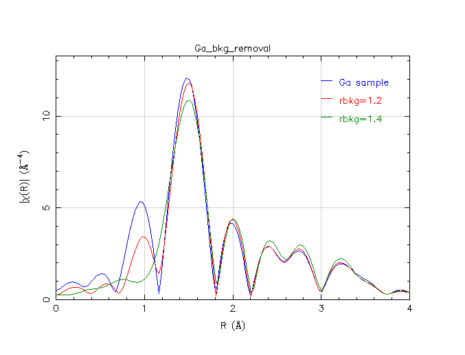
Experimenting with R_bkg

As you can see, this has an impact. Increasing R_bkg changes the cut-off in Fourier space between the background and the data. Given a bit more freedom to follow the variations in the data, the background function determined with successively larger R_bkg values does a better job of elminiating the spurious peak below 1 Å. However, as we increase the R_bkg value, the peak at about 1.5 Å is affected. Because the 1.5 Å peak is significantly attenuated by the choice of R_bkg=1.4 Å, this value may be suspect.

Changing k-weight

Changing the k-weight used in the background removal affects the evaluation of the optimized spline. Here are three background removals, all with R_bkg=1.2 Å, and with different values of k-weight.

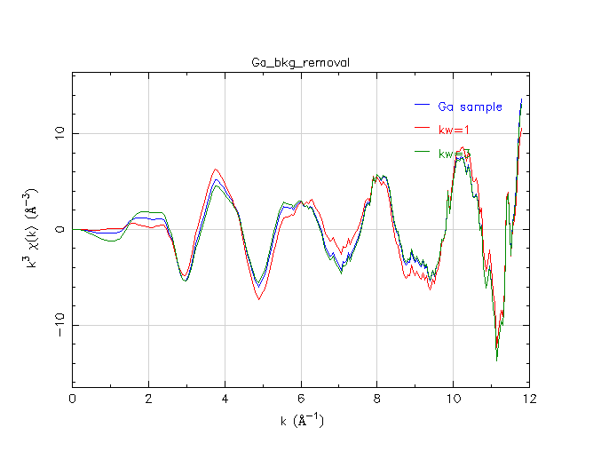
Experimenting with k-weight

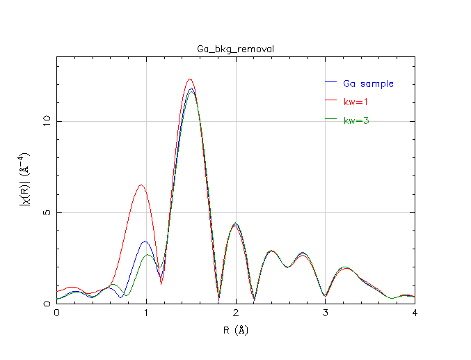
Experimenting with k-weight

As you can see, there are significant differences at low-R in how the spline follows the data using the three different k-weights. Of course, since we are performing a Fourier transform over a finite – and rather limited – range in k-space, all of the peaks in R-space are rather wide. It is impossible to completely separate peaks in R-space – the peak just below 1 Å has width that overlaps the width of the 1.5 Å peak. As a consequence, changing the peak below 1 Å by changing the k-weight has an impact on the peak at 1.5 Å. The trick is in evaluating and interpreting this impact.

Spline range and spline clamps

These two parameters also effect the background removal. One could do experiments of the sort shown above to examine these parameters as well. In practice, I tend to adjust these parameters less than R_bkg and k-weight.

Visualization matters!

All of the plots made so far have used particular values of plotting k-weight (i.e. the one from the strip below the purple plotting buttons) and particular values of Fourier transform range (i.e. the one with the blue shadow in the Athena screenshot above). How the processed data looks obviously depends on those choices as well. In particular, the Fourier transform range must be chosen sensibly. The data above 11 Å^-1 look funny to my eye. I suspect that there is some systematic problem that is dominating the data in that energy range. Above, all plots of χ(R) were made by transforming all the way out to 11 Å^-1. 10.5 Å^-1 is probably a better choice.

Choosing the “right” values

On this wiki page, I’ve discussed the meanings and effects of the various parameters, but I have not provided a recipe or proscription for processing your data. In practice, that is not really possible. There are good practices that work much of the time, but data is often fussy and requires that you fuss with it. At the end of the day, the most important thing is to remember what your goal is. Your goal is eventually to analyze your EXAFS data.

That is, you will eventually export data from an Athena project into an Artemis project. You will then do some kind of data analysis and say something about the configuration of your local coordination environment. Your goal is to say something defensible about how many atoms surround the absorber, how far away they are, and how disordered they are. The point of dtaa processing, therefore, is to prepare for data analysis and to do so in a way that does not make your analysis less defensible.

To say that another way:

Note

Your data analysis should not be strongly correlated to your data processing.

At the level of using Athena, you actually have no way, whatsoever of knowing what the “right” values of the background removal parameters actually are. The only thing you can do is process your data in a way that seems reasonable. Once you begin doing data analysis, then you are able to evaluate the quality of your data processing.

Here’s how: import your processed data into Artemis. Work on a fitting model until you think you have a decent understanding of the structure. Then, back in Athena, change the data processing parameters, reimport the newly processed data and redo the analysis. Did the values change outside of their error bars? If so, then the answers you are looking for are highly correlated with your data processing parameters. If not, then the answers you seek are mostly independent of the data processing. (Scott Calvin often refers to this as the stability of the fitting model.)

That, then, is the answer. Do your data processing in a reasonable way – remove the low R peaks as best as you can while not obviously damaging the part of the data you intend to analyze. If you can do so in a way that the results of your fitting model do not correlate strongly with the details of your data processing, then you may have found a defensible result.